The robot can pick. Now the site has to pay back.

The robot in our Retail Lab can move a predefined three-item basket through a simulated store. That is useful engineering work. It is not yet a business.

A retail operator does not buy an arm because it moves well in a render. The operator buys a system if it can cover expensive hours, remain available, and return its installed cost in a reasonable period. So we built the next simulation around that decision.

Five inputs, one gate

The interactive model asks for five assumptions:

• Staffed hours the cell could replace each week
• Fully loaded hourly labor cost
• Installed cell cost
• Annual operating cost as a share of that installed cost
• Orders served per day

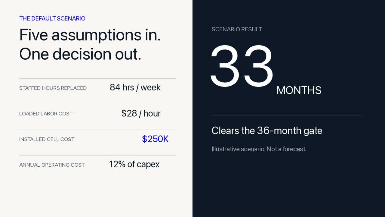
The default scenario uses 84 hours of weekly coverage at $28 an hour, a $250,000 installed cell, annual operating cost equal to 12% of capex, and 90 orders a day.

That produces $122,304 in annual coverage cost. The cell carries $30,000 in annual operating cost, leaving $92,304 in net annual labor value. Dividing the installed cost by that value gives a payback of about 33 months.

The result clears our 36-month commercial hurdle, but only narrowly. It is an illustrative scenario, not a quote, a forecast, or a measured return.

The useful result is the one that fails

Move installed cost from $250,000 to $400,000 and keep every other assumption the same. Annual operating cost rises with it, from $30,000 to $48,000. Payback moves from 33 months to about 65.

That site no longer works.

This is why the simulator is more useful than a single headline number. It shows which assumptions control the answer. A polished demo can hide a weak business case. A model that visibly fails tells us what the pilot must measure and what the hardware team must change.

For this concept, installed cost and displaced coverage matter more than raw robot speed. A faster arm does not rescue a cell that costs too much or a location that does not need enough staffed hours replaced.

The counterintuitive capacity result

At 90 orders a day across 12 hours of coverage, the default site averages 7.5 orders an hour. Against the pilot target of 60 orders an hour, that is only 12.5% capacity use.

Low use is not automatically a failure. The product is availability. The machine has to be ready when an order arrives, even if it spends most of the day waiting. The commercial comparison is the cost of that availability against the cost of keeping a person on site.

That distinction changes the engineering priority. Once the cell can serve the peak queue, pushing theoretical throughput higher creates little value. Lower installed cost, faster recovery, simpler restocking, and better uptime matter more.

What the calculator leaves out

The interactive version is a screening model, not the full unit model. It deliberately excludes financing, taxes, shrink, rent, payment fees, packaging, restocking labor, downtime, and residual value. Those costs belong in an operator-specific deployment model after supplier quotes and a real site are available.

It also treats avoided coverage as value without claiming every hour becomes a direct payroll reduction. An operator may redeploy people, keep overlap for restocking, or require human support during a pilot. Those are operating decisions, and the model should make them visible rather than quietly count them as savings.

What the pilot has to replace

The simulator gives us a list of assumptions that must become measurements:

• The installed price of the complete cell, not just the robot arm
• Service, monitoring, spares, power, and intervention cost
• Restocking time per delivery and per order
• Availability after jams, failed picks, and recovery
• Actual orders by hour, including the peak queue
• The real coverage cost at the host site

The next physical cell does not need to prove that robotics is impressive. It needs to replace those six assumptions with evidence.

Try the interactive economics model in Retail Lab.